Short Guided Introductions to iolite Essentials
Below you will find short guides to using iolite Essentials (hereafter “Essentials”). If you have never used Essentials before, we recommend starting with the first guide and then reviewing the others to gather more information relevant to your application.
1. Import Basics and Imaging Guided Intro
As this is just a short introduction to iolite Essentials, only minimal details will be included in the guide. There will be however links to additional information for further in depth discussion of certain features.
In this guided introduction, we will be using an example imaging dataset, which can be downloaded here. It is a meteorite sample measured on an Agilent quadrupole instrument, and will be processed in ‘semi-quant’ mode (i.e. without internal standards). The mass spec file is the met_1.csv file and the laser log file is the met_1_log.csv file. The .zip file should be unzipped to a location on your computer where you have full read/write access before starting the guide.
Start iolite Essentials
The first window that will appear after staring Essentials is the Welcome Window. More detailed information about the Welcome Window can be found here.
On the left of this window are the Start and Recent sections. In the Start section, there are buttons for creating a new session, opening an existing session file, or starting a new “live session”.
Note
A “live session” is where iolite Essentials is connected to AV2 Chronicle, and receives mass spec and laser metadata after each sample is completed. Live Sessions will not be covered in this guide. More information about setting up and running live sessions is available here Live Sessions
Tip
If the New Session, Open Session and Live Session buttons are greyed out, you need to start a trial or enter your licence details. See Installing and Registering iolite Essentials for more details.
Note
This guide uses the Imaging Module, which is enabled by default during the trial period. After the trial ends, you must purchase a subscription to the Imaging Module if you wish to enable these feature.
One difference between previous versions of iolite and Essentials is that in Essentials all data and log files are loaded at the beginning. There is no option to add data after the import step (unless you’re running a Live Sessions). The laser log file should be in the same folder as the mass spec data, and Essentials will look through the folder and find all the mass spec files and laser log files.
Warning
Essentials requires a laser log file to process results. The laser log file must be created as the experiment runs as they cannot be created after the experiment. See here for instructions on creating laser log files.
Import your data
The import process involves:
selecting the folder containing your data,
syncing the data,
assigning samples to groups, and finally,
selecting baselines.
Click the New Session button to start the import process. Essentials will prompt you to open a folder containing both the mass spec data files and laser log files (Fig. 11).
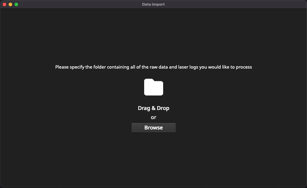
Fig. 11 A screenshot showing the first window in the import process
Once a folder is selected the Synchronisation Window will appear (Fig. 12).
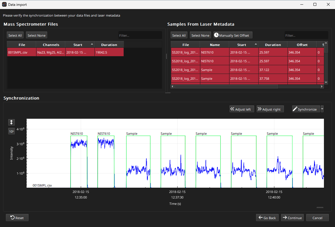
Fig. 12 A screenshot of the Synchronisation Window
The upper half of the Synchronisation Window has two lists: the left for mass spec files, and the right for laser log samples. By default, all mass spec and all laser log samples are selected. In the bottom half of this window, there is a plot to show the results of the synchronization.
Depending on whether you’ve used Essentials before, there may be an exclamation mark next to the mass spec file (001SMPL.csv) in the list of mass spec samples. As we are loading an Agilent file which has a non-specific timestamp format, we may have to set the timestamp. In this case we can simply right-click on the file and select “Reprocess with automatic format”. This will cause Essentials to re-import the file and guess the timestamp format. Normally you would set the timestamp format for your lab and not have to change it again. After selecting to reimport with automatic format, the exclamation mark next to the file name disappears and the list of channels is populated, as is the plot in the lower half of the window.
With both the mass spec file selected, and all the laser log files selected, click on the Synchronize button at the top right of the plot. You can zoom the x axis of the plot with the mouse scroll wheel. Zooming in will show that the laser log and mass spec data are now synchronized. The Offset in the list of laser log samples should now also show an offset of ~346 s.
More detail about the Synchronisation Window is available here.
Click the Continue to assign samples to groups.
Assigning samples to groups
In the Sample Destination Window (Fig. 13), the groups that will be created and which group each sample will be assigned to is displayed. In this example, we have just two groups: “G_NIST610” for our NIST 610 analyses, and “Sample” for our image scanlines. Essentials uses the sample name recorded in the laser log file to determine which group to assign each analysis to.
There is not much we need to do in this window as the groups have been automatically set up correctly. We’ll just set the start and end crops for NIST610 analyses to 1 s, respectively. We won’t crop the image scanlines. To do this, type “610” in the filter at the top right of the Samples Table. Then select all samples in the table by clicking on any sample and pressing Ctrl + a (Cmd + a on Mac). Then click the Set Crops button and enter 1 for both the start and end crops. The table will now be updated with the crop times (you may have to scroll the table to the right to see the crop times columns).
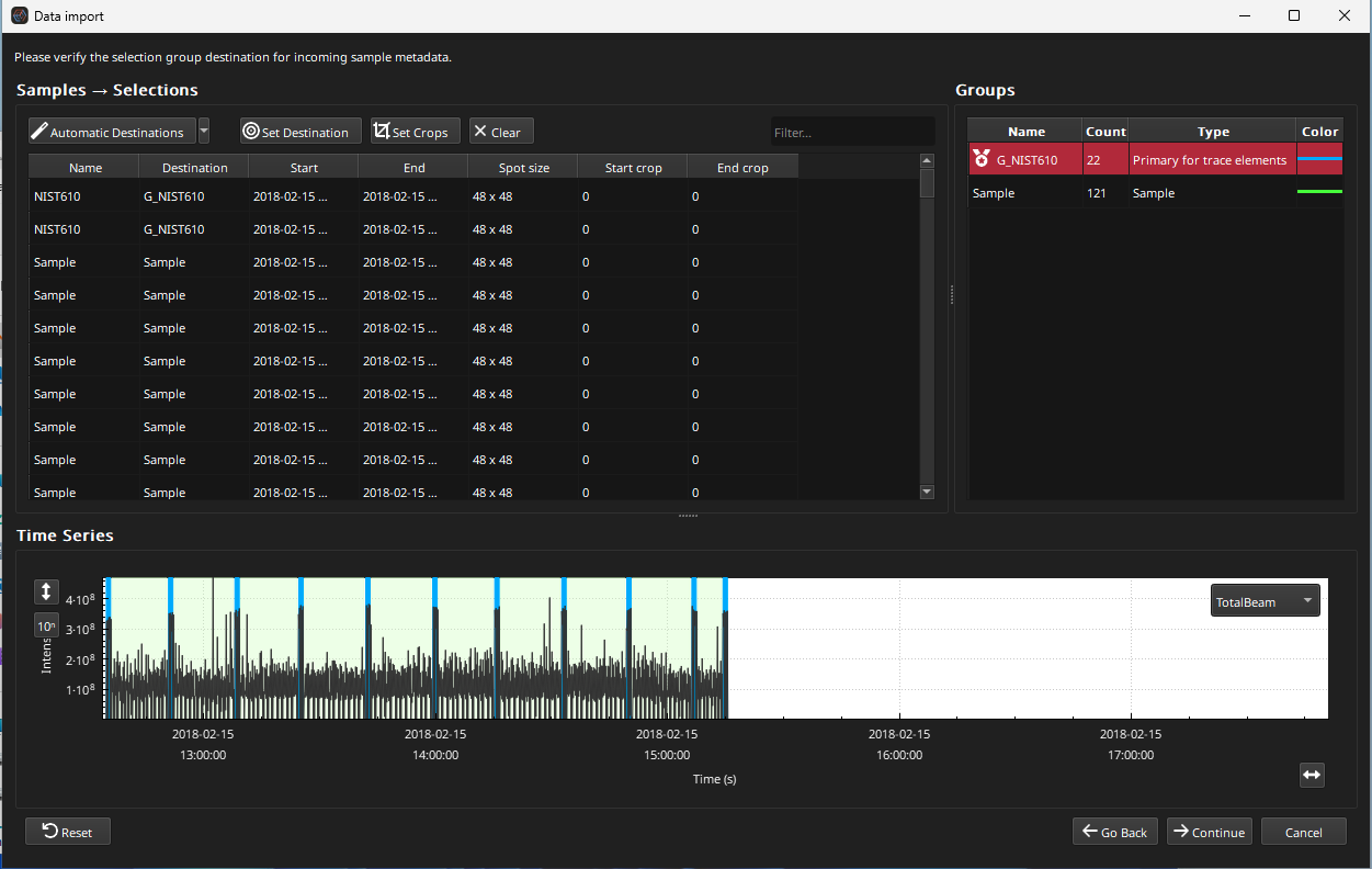
Fig. 13 A screenshot of the Sample Destination Window
More detail about the Sample Destination Window is available here
Click the Continue button to continue to the Baseline Settings window.
Settings up baselines
The Baseline Settings Window visually sets the intervals iolite will use to interpolate baseline signals. You can zoom in on the intervals between ablations using the mouse scroll wheel. Zoom in until the baseline signals for a few ablations are clearly visible. Change the Wash In setting to 2 s and the Wash out setting to 2 s. Set the minimum duration to 3 s. This should result in the baselines being selected without much wash-in or wash-out affecting the selected intervals.
If the baseline spline type is ‘Spline - AutoSmooth’ you may receive a warning at the top that the fit is ‘bad’. This is due to the very long interval at the end of the experiment where no samples were measured. Due to the spline fit, the baseline spline is unconfined in this interval and is very steeply positive. This could result in very abnormal baseline subtracted values, hence the warning. However, in this case there are no samples in this region and we can ignore the warning. Alternatively, the Interpolation method could be switched to “Step forward” so that there is no unconfined spline effects at the end of the experiment.
More information about the Baseline Settings Window is available here
Click the Import button to finish the import process. The main Essentials window will appear.
Main Essentials Window
After the import process is completed, the main Essentials Window will appear (Fig. 14). This window shows the results of the experiment arranged as a table, with selections/samples as rows and channels as columns. All selections are arranged in groups, starting with baseline selections at the top, then reference materials, and finally unknowns. Each group can be expanded by clicking the small arrow to the left of the group name.
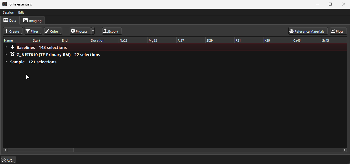
Fig. 14 A screenshot of the Sample Destination Window
By default, Essentials will automatically calculate all results for all modules enabled, as long as there is enough information for it to do so. In this case, we have all the essential pieces of information required to calculate trace element results: baseline selections and primary reference material selections (G_NIST610 in this case).
Tip
If you have used Essentials before running this guide, you may have switched on the “Use Int Stds” option. When this option is selected, Essentials will use internal standards to calculate “full quant” trace element concentrations (explained in Paul et al., 2023). To quickly unselect this option, click the down arrow next to the Process button. This shows processing options. Deselect the “Use Internal Standards” option as we do not need it for this example.
Clicking the arrow to the left of each group name expands the group to show the selections within that group.
By default, all input, intermediate and output channel columns are shown (along with some metadata columns such as start time, end time and duration). You can quickly filter this table to show only the output channels by clicking the Filter button and clicking the Output button in the Channels options. The table columns will update to show the metadata and output columns. In this case, these are the ppm channels (i.e. output channels). If these columns are blank, see the tip above about unchecking the “Use Internal Standards” option.
In this example, each selection is actually a scan line, so the mean concentration for each selection is less interesting than the images that will be created. More detail about the Main Window will be presented in the following tutorial. Alternatively, documentation for the Main Window is available here.
If the output channels have non-zero entries, we can continue to creating images in Essentials.
The Imaging Tab
In the top left of the main window there are two tabs: Data and Imaging. Click on the Imaging Tab (noting that the Imaging Module is a separate subscription module and must be purchased after the trial ends). A screenshot of the imaging tab is shown in Fig. 15.
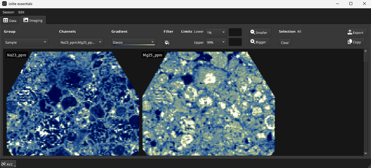
Fig. 15 A screenshot of the imaging tab in iolite Essentials
The Imaging Tab is discussed in more detail here. At the top of the Imaging Tab are controls for which images to show and how to color them etc. Click the Group drop-down menu to select our Sample group. In the Channels drop-down menu, go to the Output channels, and click the Toggle All button at the bottom of the list. An image for each Output channel will now be created in the main part of this tab.
By default, all images are selected. Clicking on any image will then select that image. Which image is selected is shown in the top right of the tab (labelled ‘Selection’). To select all images, click the Clear button beneath the ‘Selection’ label or click on any blank part of the main part of the tab.
Set the color gradient limits to 1% and 99% using the Limits drop down menus.
You can change the color gradient used to color the images using the Gradient dropdown menu.
Double-clicking on any image will show the individual image in more detail. When an image is shown in detail, clicking the < or > buttons (top left) moves between images. Selecting an image from the drop-down menu in the top left also changes the image shown. The palette button toggles whether the color scale is shown to the left of the image.
Clicking the button will return the display to all images.
With all images displayed, the Smaller and Bigger buttons will decrease/increase the size of the images shown (this does not affect the underlying data resolution, just the preview image size).
Image Export
Clicking the Copy button will copy all images to the clipboard.
Clicking the Export button will show the export dialog (shown in Fig. 16).
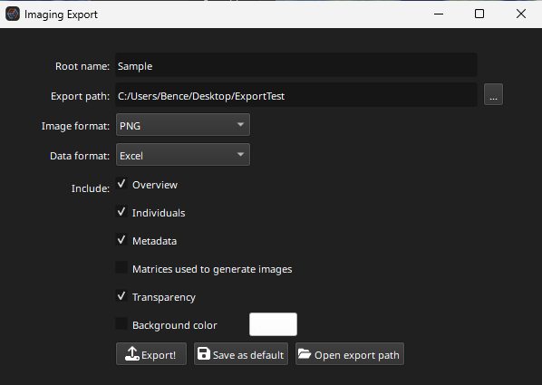
Fig. 16 A screenshot of the export dialog of Essentials’ imaging tab
The root name is a prefix added before each image. For example, if the root name is ‘Sample’, the images saved will be ‘Sample_Na23_ppm’, ‘Sample_Mg25_ppm’, etc.
To select the folder to export the images to, click the … button at the end of the Export Path field. Create a new folder to store the images that will be exported.
The Data format menu selects the format of the file describing the imaging metadata (e.g. image and spot dimensions).
Change the image format to .png and click the Export! button. At the top right of the main Essentials window a small progress indicator will appear showing the export progress. Wait for it to reach 100%, then click the Open Export Path button to show the exported images.
This concludes this short guide showing a simple imaging experiment processed in Essentials. To continue to a spot analysis trace element example, click here. To continue to a U-Pb geochronology example, click here.
2. Trace Elements Example with Internal Standards
This guided example will show you how to process spot analyses with internal standard values. It uses the Gabbros dataset, which can be downloaded from here. The .zip file should be unzipped to a location on your computer where you have full read/write access.
This is a spot analysis dataset, collected on an Agilent mass spectrometer. The example files include the mass spec data (Gabbro_data.csv), laser log file (Gabbro_log.csv) and a file containing internal standards (IntStd) values measured by electron microprobe (Gabbro_IS_values.xlsx) in units of elemental weight percent. No geological knowledge is assumed for this tutorial, although the following context may be useful.
A gabbro is a course-grained volcanic rock, and in this experiment we measured the following mineral types:
Olivine (a Mg and Fe bearing silicate, labelled “Oliv” in the experiment)
Clinopyroxene (a silicate mineral containing significant amounts of Ca, Mg and Fe, labelled “Cpx”)
Plagioclase (A Na Ca bearing silicate, labelled “Plag”)
Titanomagnetite (an Fe oxide, labelled “Opaq” as it is opaque to transmitted light).
Each analysis is labelled as one of the above groups (“Oliv”, “Cpx”, “Plag” or “Opaq”) although there are one or two mis-labeled analyses and drill-throughs. Finding these is left to the reader as an exercise in checking results.
Three reference materials were analysed in the experiement: NIST 612, BCR2G and BHVO 2G. The latter two are basaltic glass RMs and no additional information about these is required except to note that they are more closely matrix-matrix to some of the minerals were are analysing in this experiment. More information about each can be found here and here, respectively.
Import the data
Start a new session, and select the folder containing the example data. If there is an exclamation mark next to the mass spec file name, right click on it and select “Reprocess with automatic format”. Click the Synchronize button. The offset for all samples should be approx. -271 s. In the Sample Destination Window, NIST612 should be automatically selected as the primary for Trace Elements. If not, double click on the G_NIST612 group’s entry in the Type column and select “Primary for trace elements.”
There should be a separate group for clinopyroxene (Cpx), olivine (Oliv), opaques (Opaq) and plagioclase (Plag) analyses. Click on each group to see where they occur within the experiment.
Set the start and end crops to 1 s for all analyses using the Set Crops button.
Wash-in and Wash-out times of 2 s each should work well. Click Import to finish the import process.
Setting Internal Standard values
The Main Essentials Window is divided into samples as rows, and channels as columns. Expand a group to see results for samples within the group. By default all channels are shown. This includes Input, Intermediate and Output channels. Input channels are the raw data imported from the mass spec data file, and are not changed by Essentials in any way regardless of how many times or how many different ways the data are processed. Intermediate channels are channels used in the calculation of the final results. Typically, intermediate channels include things such as baseline subtracted value (channels with the suffix “_CPS”), raw ratios and similar intermediate values. Output channels hold the final results for each sample, such as concentration values (channels with the “_ppm” suffix) and final ratios for geochronology.
All this information is provided to aid the analyst in checking the results and ensuring the data are correct. For an initial inspection however, it is typical to view the Output channels first. The columns shown can be filtered using the Filter button (top left). The options this displays are shown in Fig. 17.
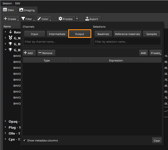
Fig. 17 A screenshot showing the options displayed by the Filter button
To show just the Output channels, click the Output button (top center of this dialog, highlighted in orange in Fig. 17). Now only the _ppm channels will be shown in the table.
By default, there should be non-zero values for the Output channels. These have been calculated with the information provided so far: baseline selections, RM and unknowns selections. These have been calculated using a ‘semi-quant’ approach (this term is explained in Paul et al., 2023). To add internal standardisation, click the down arrow next to the Process button, and check the “Use Internal Standards” option. Three new columns will appear in the table:
Internal element (the element to use for internal standardisation)
Internal value (the concentration value to use)
Internal units (the concentration units: note weight percent is abbreviated to “wtpc”).
Double clicking in the entry corresponding to a sample will set the value for that sample. For Internal element and Internal units, double-clicking will show a drop-down menu with available options.
Tip
Double-clicking on a value also opens the Plots panel. This panel can be closed again by clicking the Plots button in the top right of the main window. The Plots Panel is described briefly below, and in more detail here.
Setting the Int Std values for each sample manually like this would be very time consuming. Setting Int Std values for an entire group can be accomplished by right-clicking on a group’s name shows the Context Menu. Note that right-clicking on a sample’s name will also open the Context Menu, but we want to set the values for all samples within a group at once by right-clicking on the group name. In the Context Menu, select the Setup -> “Set internal standard” option. This will display the dialog shown in Fig. 18. This dialog shows options for setting the element (channel), the concentration units, and the concentration value. If the group clicked on is an RM the concentration will be automatically filled by Essentials. All Int Std values will be entered for the entire group. Use the context menu to set the Int Std element to Ca43 for the three RM groups.
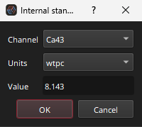
Fig. 18 A screenshot of the internal standards dialog from the context menu
This is a good approach if all samples within a group have the same Int Std value. In this dataset however, each sample has a different Int Std value, and we will use more than one element as internal standard (Ca and Ti in this case). To set multiple elements and concentrations open the file in the example dataset called “Gabbro_IS_values.xlsx”. This file shows the Ca and Ti values measured by electron microprobe (other elements measured were omitted from this file). In columns G, H and I, the data have been arranged as they should appear in the Essentials data table. That is, Int Std channel, then concentration value, and then units. Copy these data from the Excel file. In Essentials click in the Internal Element column, in the first row of the Cpx group, and press Ctrl + v (Cmd + v on Mac) to paste the Int Std values into the table. The Int Std values for all reference materials and unknowns has now been set and there are now concentration values in the Output channels that use these Int Std values.
Tip
The “Internal element” column needs the name of an Input channel, not an element. For example, in this dataset we need to ensure “Ca43” is entered rather than just “Ca”.
Simple QAQC
Essentials offers many tools for interrogating your data. This guide will look at just a few examples, but one of the first tasks in checking your data is to view QAQC data.
In our example, G_NIST612 is the primary reference materials. This leaves BCR 2G and BHVO 2G as secondary reference materials for checking our data reduction process is valid. Essentials will automatically provide a QAQC report for each secondary reference material. To view the QAQC report for a secondary reference material, right-click on the group’s name, and select View -> “QA/QC” from the Context Menu. This will display the QAQC report for this group. An example is shown in Fig. 19.
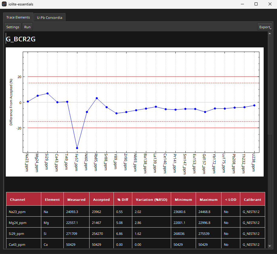
Fig. 19 A screenshot of an example QAQC report from the Gabbros example dataset
The QAQC report can be saved either as a PDF file or HTML file by clicking the Export button in the top right of the QAQC window. Settings can be changed via the Settings button (top left) and the report can be re-run by clicking the Run button (top left). More detail about this QAQC report, including how the values are calculated, is available here.
One quick statistic to help gauge the overall performance of a data reduction process (beyond looking at individual elements) is to look at the sum of all the differences between the accepted value and the mean measured value. This sum is placed in the bottom of the QAQC report and labelled “Sum of Abs % Diffs”. Using NIST612 as the primary RM, this statistic is 159%.
Changing Primary Reference Material
The values for BHVO 2G in this example experiment look OK, but let’s see how they change when we use BCR 2G as the primary reference material. To change primary reference material, right-click on the new primary RM (in our case G_BCR2G), and select Setup -> “Use primary trace elements primary” from the Context Menu. You should see that the icon beside G_BCR2G is now a medal (indicating that it is the primary reference material) whereas the icon next to the other RMs is a to indicate that they are secondary. The results should be automatically recalculated. If not, check that the “Re-crunch on change” option in the Process button menu (accessed by clicking the down arrow next to the Process button) is selected.
Checking the QAQC results for BHVO 2G with BCR 2G as the primary reference material shows that the sum of absolute percentage differences is now ~64%. This is because the matrix of BHVO 2G is more similar to BCR2G than NIST612.
Creating and Deleting Selections
The terms selection and sample in this guide have been used somewhat interchangeably. This is because up to this point, each sample in the laser log file was use to create a selection. However, in Essentials (and iolite more generally) you can adjust the interval used to calculate results for a sample. This adjustable interval is known as a selection, whereas the sample is interval defined in the laser log file.
This example will demonstrate how to create a selection where there is no sample. In this example dataset (and in general), it would be beneficial to have an additional baseline selection after the last analysis (the last NIST612 analysis in this example) to help confine our baseline spline.
Click the Create button (top left of main window) and select “Selections”. The Create Selections dialog (Fig. 20) will appear.
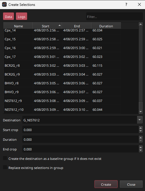
Fig. 20 A screenshot of the Create Selections dialog
In the Create Selections dialog, new selections can be created based on the mass spec (‘Data’) and laser log (‘Logs’) samples. In this case, the selection to be created will be after the last Log sample. Scroll to the bottom of the list and select the NIST612_r10 sample. Change the Destination group to “Baselines” (it should auto-complete the group name). Set the Start Crop to 63 s and the Duration to 30 s. The End Crop will remain 0 s and will be ignored in this case. These settings will create a selection that starts 63 s after the last ablation starts, and will have a duration of 30 s, as shown diagrammatically in Fig. 21.
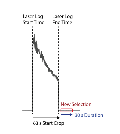
Fig. 21 A diagram showing how start crop times can be used to skip the entire ablation
Turn off the Output channels filter in the Filter menu by clicking Output again. Expanding the Baselines group will show this newly created selection at the end of the list of selections (it has a duration of 30 s when most other baseline selections have durations or ~22 s).
To delete a selection, right-click anywhere in the selection’s row, and from the context menu select Edit -> “Delete Selections”.
Plots and Spline Mini-graphs
Double-clicking on any result will open the Plots Panel. Clicking the Plots button (top right of main window) will also open/close the Plots Panel. In the top plot (the “Time Series” plot) the highlighted selection can be viewed in the context of the time series, and adjusted manually if required. The middle plot shows means and uncertainties for selections within the current group, with the currently highlighted selection in red. Double-clicking a result in this plot will highlight it in the main data table, and show it in the Time Series plot. The Concordia plot is covered in more detail in the U-Pb example. More detail about the Plots Panel is available here.
Typically, result outliers can be identified either via coloring of the data table (described below) or using the Plots Panel. However, sometimes smoothed splines can behave in undesirable ways where they do not smoothly represent the data. One common example of this is two selections very close in time with very different values. The spline will attempt to pass through both values, but this may lead to very large curvatures in the spline surrounding these points. One way to spot this is via the spline mini-graphs, shown at the bottom of each baseline or reference material group. Two examples are shown in Fig. 22.
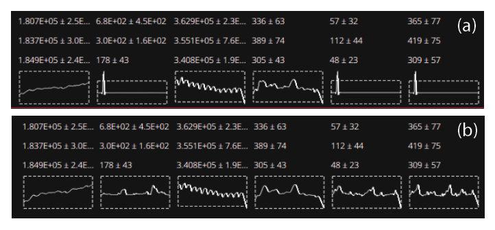
Fig. 22 Two examples of spline mini-graphs in iolite Essentials. The upper panel (a) shows splines with anomalies, most obvious in the second, fifth and sixth channels. The lower panel (b) shows the same data but with the selections adjusted to avoid the anomaly. More details about this process in the text.
The spline mini-graphs show the spline for each channel, within the context of the group average for that channel, the latter shown as a dashed rectangle. The upper and lower edges of the rectangle show the mean ± 2SD of the group results. Splines that extend significantly beyond this rectangle should be inspected for outliers, or for results very close in time but with significantly different values. The upper panel in Fig. 22 shows an example where two baseline selections were improperly adjusted so that they included some ablation intervals. The lower panel in Fig. 22 shows the same data with the selections correctly adjusted. The spline in the lower panel stays within the bounds of the group stats box, although at the very end of the experiment (right side of the spline mini-graphs) it does trend sharply lower for some channels. Adding the final selection as described in the previous section avoids this sharp downward trend.
Changing Spline Type
The default interpolation method in Essentials if there are more than three results in a baseline or RM group is a smoothed cubic spline. However, there are times where this might not be the most appropriate interpolation method. To change the interpolation method for a group, right-click on the group and select different interpolation method from the Setup -> “Spline type” menu in the contenxt menu. Checking the QAQC report for a secondary reference material is a good way to test the effect of changing a spline type.
Further Inspection of Data
Beyond QAQC and the Plots Panel, there may be more subtle variations in our results that we would like to be aware of. One option for this is to use the data table color formatting options built into Essentials. Clicking the Color button of the main window (top left). The most basic of these is to color the the groups according to type to help differentiate between RMs and unknowns, and between Input, Intermediate and Output channels. These options are available using the “Highlight Channel Types” and “Highlight group types” in the Color menu.
Sometimes it can be easy to miss an unusual result in a data table with many results displayed at once. To help identify clearly outlying results in our data table, the “Group/outliers” Mode can be chosen from the Color menu. This mode will automatically highlight results that are greater than 3 SD from the group mean. An example of this can be seen by viewing the Zr90_ppm channel for the Plag group (Fig. 23). The second analysis should be highlighted as an outlier. Double-clicking this result to show it in the Plots Panel reveals the plots shown in Fig. 24. This analysis likely represents a “drill through” can be corrected by adjusting the right side of the selection (red rectangle) in the Time Series plot so that it doesn’t include the drill through (i.e. excluding the last part of the data). After adjusting, the Stats plot should show that this sample now has the same average as the other analyses in this group.
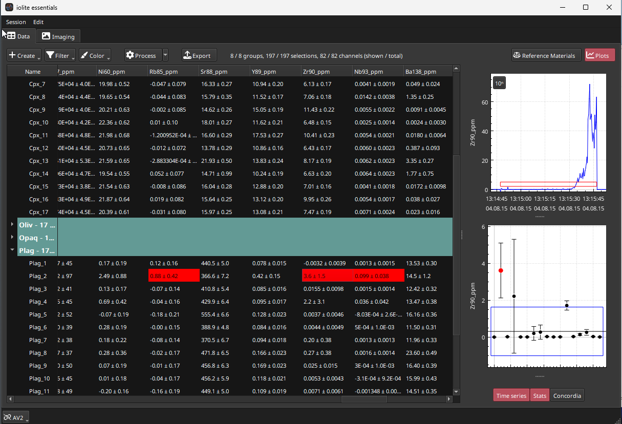
Fig. 23 A screenshot from Essentials showing outlier highlighting
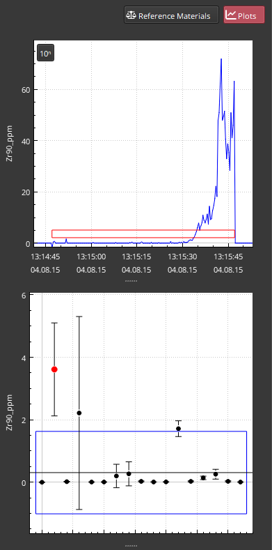
Fig. 24 A screenshot of the Plots Panel in the example dataset showing an outlier result possibliy due to drill-through
Another option for highlighting the variation in the result is to select the “Group/channel” option from the Mode dropdown menu of the Color button. This mode will color each cell in the data table according to their value within the group with the lowest values being colored with the lower colors in the color gradient and the highest values in the group being colored with the highest colors in the gradient. The color gradient can be set in the Color button menu. In this example dataset, using this color mode will highlight the Plag_12 selection in channels such as Y89_ppm. All other samples in this group have low values, but Plag_12 has a high result, and this results in the cells all having one low color but Plag_12 having a lighter color. Clicking on the Y89_ppm cell for this sample shows that this was likely a misplaced spot, with the spot area possibly overlapping with a different mineral (Fig. 25). Adjusting the selection in the Time Series plot to the last part of the ablation brings this result back in line with other analyses in this group. Alternatively, this analysis could be deleted by right-clicking on the result and selecting Edit -> “Delete selections”. Doing this will result in a prompt asking if you want to delete the chosen selection. Clicking OK will confirm the deletion. This deletion can be undone by selecting the “Undo” item in the Edit menu.
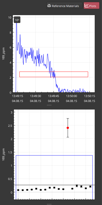
Fig. 25 A screenshot of the Plots Panel in the example dataset showing an outlier result possibliy due to a misplaced spot
Finally, the “Selection/channel” color mode shows the values within each selection as slices in an elongate rectangular plot. Again, this can be useful for finding spikes in data that may not be obvious. An example here is Plag_5 in the Ti49_ppm channel. Most of the rectangular plot is low colors, with a single time-slice appear as a high color. It should be noted however that this single value would be excluded from the result for this sample as an outlier, and that adjusting the selection to exclude this spike has little effect on the calculated result (because it is already outlier rejected).
Note
You can adjust outlier rejection settings in Essentials’ preferences, in the Statistics section.
Data Export
Once QAQC and selection adjustment has been completed, the data can be exported. Clicking the Export button will show the Export Options dialog (Fig. 26). A typical set of options is shown in Fig. 26.
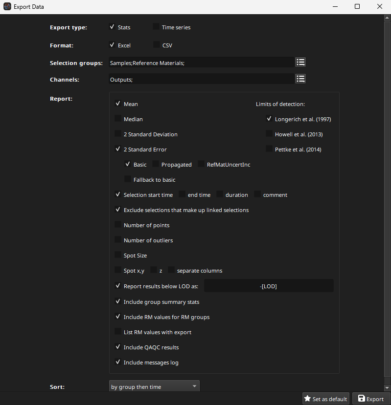
Fig. 26 A screenshot of the export options dialog, showing a typical set of options
Once you have selected the options for your export, you can save the format etc as the default by clicking the Set as Default button at the bottom right of the dialog. To export your results, click the Export button. Essentials will prompt you for a save location, and save your results.
This concludes this guide to trace element concentration processing with Essentials, using internal standards, checking results with QAQC reports and using results coloring to find outliers etc.
If you have any questions about this example, or about Essentials in general, please let us know at iolite’s support email, or on iolite’s forum.
3. U-Pb Example
The example dataset for this guide is the DRO4 zircon dataset, which can be downloaded here. The example dataset comprises one mass spec file (DRO4.csv) and one laser log file (DRO4_log_20180731_130249.csv). The .zip file should be unzipped to a location on your computer where you have full read/write access.
Please note that the U-Pb Data Processing Module can be purchased as a separate module after the trial ends.
It is recommended that you have completed the 1. Import Basics and Imaging Guided Intro guide before starting this guide. It also assumes you are familiar with the concepts presented in this webinar.
Importing the data
In Essentials, start a new session either from the Session menu or from the Welcome Window. Select the folder containing the mass spec and laser log files. If you haven’t changed your Agilent timestamp format, it is likely that you will see an exclamation mark next to the mass spec file in the Synchronization Window. This indicates that use timestamp format currently saved could not be used. To fix this, right-click on the DRO4.csv file in the Mass Spec Files table. Select the “Reprocess with automatic format” option. Essentials will automatically determine the correct timestamp format, and the file should be imported correctly. The exclamation mark beside the DRO4.csv file listing should disappear and the synchronization plot should show the mass spec data. Click the Synchronize button; the offset should be approximately 77 seconds for all samples. Click the Continue button.
In the Sample Destination Window, change the Type for Z_91500 to “Primary for U-Pb” and change the Type for Z_Plesovice to “QA/QC”. Select all samples in the Samples Table by clicking in the table and pressing Ctrl + a (Cmd + a on Mac). Set the start and end crops to 1 second using the Set Crops button. Click the Continue button.
This example file has a washout artefact, with a smaller peak arriving after the main washout. Increase the “Wash out” value to 16 s, and set the “Wash in” value to 1 s. Set the Minimum duration to 0 s. Click the Import button to complete the import process.
Viewing the Results
For this dataset, we don’t want to use internal standards, so they can be unchecked in the Process button options. Filter the table to show only the Output channels by clicking the Filter button, and clicking the Output channels button.
Check the downhole fractionation fits for the primary RM (91500 in this example) by right clicking on the 91500 group and selecting QAQC from the View sub-menu. The QAQC window should look similar to Fig. 27. There are three tabs at the top of the window. The right-most tab has the downhole fractionation plots. The U-Pb Concordia plot cannot be used because this is the primary reference material.
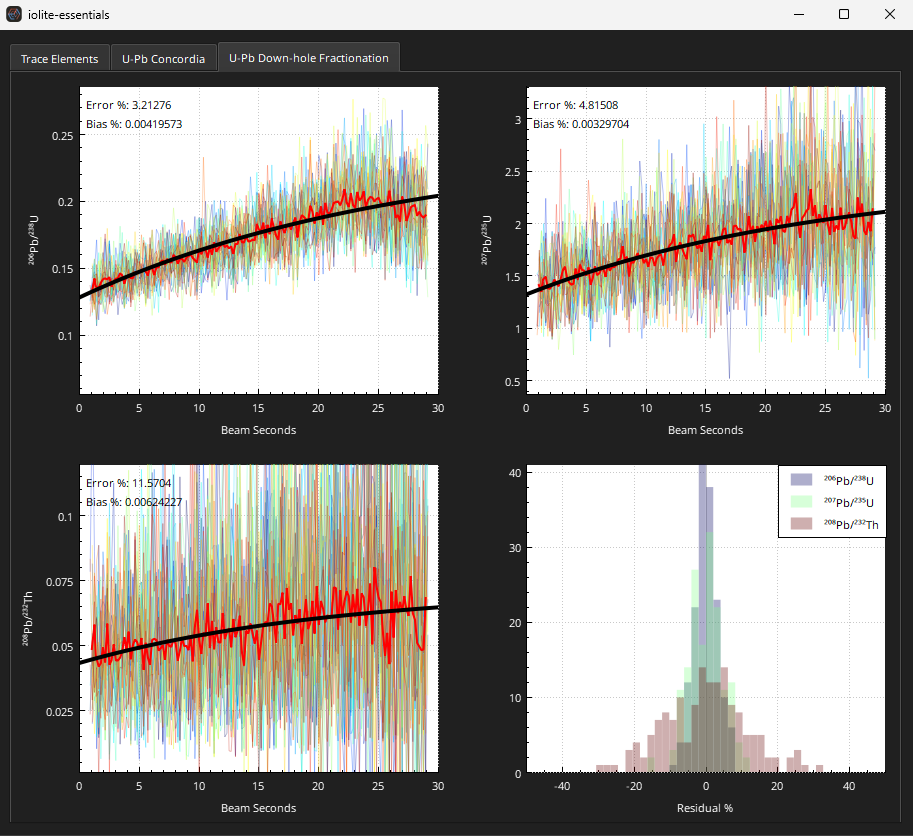
Fig. 27 A screenshot of the downhole fractionation plots in the QAQC window of iolite Essentials
The QAQC results for the secondary reference materials (Plesovice and Temora 2 in this example dataset) can by checked by right-clicking on the group name and selecting View -> QA/QC. The average measured age should be very close to the accepted age for both secondary RMs, but the plot for the Temora2 results is dominated by one analysis. This is a missed spot and can be easily identified by coloring the table using the Group/channel mode of the Color menu (see Further Inspection of Data for more examples of coloring the table to find anomalies). The second selection in the Temora2 group appears to be a missed spot and can be removed by right-clicking on the row and selecting “Delete Selections” from the Edit sub-menu. The QA/QC Concordia plot of Temora2 should then look like Fig. 28.
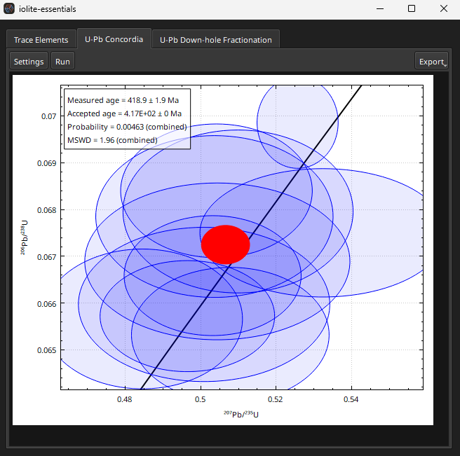
Fig. 28 A screenshot of the Concordia plot in Essentials QAQC window
Adjusting the selections
The Concordia plot of the Plots Panel can be used to adjust unknowns selections. If the Concordia plot is not shown in the Plots Panel by default, it can be turned on by clicking the “Concordia” button at the bottom of the Plots Panel. Double-clicking on a result in the Concordia plot will select that sample in the table and in the Time Series and Stats plot. The Time Series plot can be used to manually adjust the selection, in conjunction with the Concordia plot. To keep the current level of zoom in the Concordia plot, right click on the plot and select “Resize” -> “None”. More detail about the Plots Panel is available here.
Data can be exported using the same approach discussed in the Data Export section except that in the case of U-Pb data, the Propagated uncertainty should be used.
Conclusion
This concludes this guide to U-Pb data processing with Essentials. If you have any questions about this example, or about Essentials in general, please let us know at iolite’s support email, or on iolite’s forum.
4. 3D Trace Elements Example
This guided example will show you how to process trace element data with multiple reference materials calibration using the 3D Trace Elements (hereafter ‘3DTE’) approach. It uses the same Gabbros dataset as the second tutorial above. This dataset can be downloaded from here. The .zip file should be unzipped to a location on your computer where you have full read/write access. There is introductory information about this dataset in the 2. Trace Elements Example with Internal Standards example. You should have already completed the first and second guided tutorials before starting this tutorial. This tutorial also assumes you are familiar with the concepts presented in this webinar and/or this article.
Note
The Essentials’ version of 3D Trace Elements does not include the downhole fractionation correction or affinity correction that are available in the iolite v4 version of the DRS.
Please note that the 3D Trace Elements Module is available for purchase after your trial ends.
In this example we will use two reference materials (NIST612 and BCR2G) for calibration and use BHVO-2G to check our results.
Before you begin…
When running your own multi-reference material experiments we recommend that you arrange your primary and secondary RM run order similar to that shown in the Fig. 1 in Paul et al. (2023). This will simplify assigning RMs to blocks etc.
Import and Setup
Follow the same steps as 2. Trace Elements Example with Internal Standards for importing the data.
Initially, NIST612 will be selected as the only primary RM (also known as a calibrant), and if this is the first time you’ve run Essentials Int Stds will have been set to Ca43 = 1 wt%.
Tip
The default Int Std values, along with other default data processing values, can be viewed and set in Essentials’ preferences, in the Data Reduction section.
In this example dataset we want to use both NIST612 and BCR2G as our calibrants. Setting calibrants, along with the fit models and whether to force the calibration curve through zero, is accessed via the ‘3D Trace Elements Setup’ item in the Process button menu, or alternately, by right clicking on a RM group name, and selecting ‘3D Trace Elements’ from the Setup menu. The 3DTE Setup window is shown in Fig. 29.
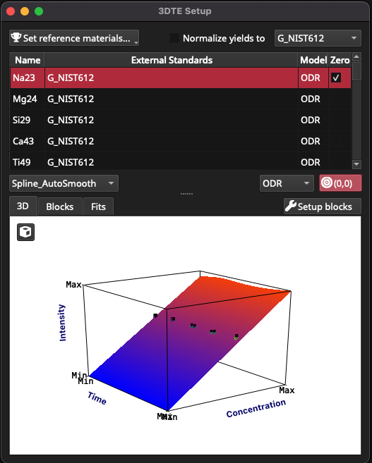
Fig. 29 A screenshot of the 3DTE Setup window
The 3DTE window is comprised of:
the ‘Set Reference Materials’ button in the top left
the ‘yield normalise’ controls (checkbox and dropdown menu) in the top right
a table of channels in the upper half of the window
controls for fitting in the center of the window (spline type dropdown menu, fit model and ‘force fit through 0’ button), and
information plots in the bottom half of the window.
The information plots include the 3D, Blocks and Fits tabs. At the top right of the information plots is the Setup Blocks button, which is used to assign RM measurements to blocks.
In this example, by default only NIST612 has been used for calibration. Because this is a single point and we haven’t selected the option to force the fit through the origin, there will be nothing initially plotted in the 3D plot. To add BCR2G to the list of calibrants for all channels, begin by clicking in the channels table (upper half of window) and pressing Ctrl + a (Cmd + a) to select all channels. Click on the ‘Set reference materials …’ and select BCR2G. BCR2G should now appear as a calibrant in the channels table, and plots should appear in the 3D plot.
Click on the Blocks tab to inspect the fits for each block of RM measurements. In this example the calibrants are a sodic glass and a basaltic glass, which are known to have different ablation properties and therefore different yields. Yield refers to the ablation efficiency of a material and can effect calibration curves/surfaces. In this example, clicking on the Ni60 channel will show an example where forcing the fit through 0,0 and applying a yield normalisation can improve the calibration curve. Fig. 30 shows the calibration before forcing through zero. Click the (0,0) button for force this fit through the origin. Check the box to the left of ‘Normalize yields to ‘ to turn on yield normalisation, and select G_BCR2G from the yield normalisation dropdown menu (top right of window). Applying this corrections improves the fit, and the Pearson Correlation Coefficient increases from 0.945 for this block to 0.996 (Fig. 31).
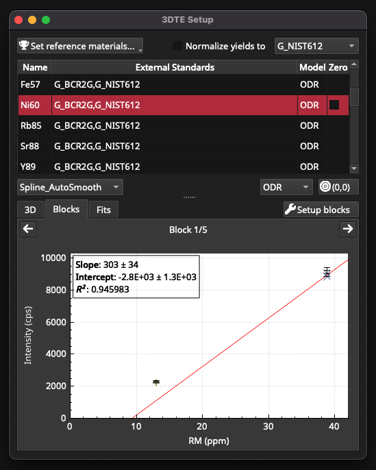
Fig. 30 A screenshot of the 3DTE Setup window showing Ni60 calibration, prior to forcing the fit through zero and applying yield normalisation
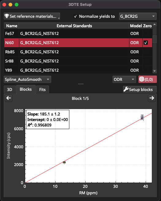
Fig. 31 A screenshot of the 3DTE Setup window showing Ni60 calibration, after applying a fit through zero and yield normalisation
Yield normalisation is applied to all channels. Forcing the fit through zero is applied on a channel by channel basis. In this example dataset, the following channels could be considered for forcing the fit through zero: Si29, Ca43, Ni60, Rb85, Y89, La139, Pb208, Th232 and U238. Any channel that has an intercept significantly below zero should be forced through zero. Any channel with a significant positive intercept (i.e. > a few 100 CPS) where no interference is suspected should be considered for forcing through zero.
Options for the fit model are provided by the model dropdown menu (immediately left of the (0,0) button). By default, the model is ODR (orthogonal distance regression) but OLS (ordinary least squares), WLS (weighted least squares), RLM (robust linear model) and York fit models are also available. See Paul et al and references therein for more details about these fits, but in practice usually an ODR, OLS or WLS fit will produce very similar results and are the typically recommended fit models.
Clicking the Fits tab shows how the sensitivity (gradient of the calibration curves) changes throughout the experiment.
The 3D plot shows how the gradient and intercept are interpolated between RM blocks. The spline dropdown menu (immediately above the 3D, Blocks and Fits tabs) provides options for interpolation between RM blocks. Using a mean or median interpolation is the same as a traditional calibration curve (i.e. one curve used for the entire experiment).
Clicking the Setup Blocks button shows how RM measurements have been assigned to blocks (Fig. 32). In this experiment, due to the way the experiment was set up, the RM measurements have automatically been correctly assigned to blocks. If this is not the case, blocks can be manually assigned or using a slightly more complex clustering approach (Paul et al., 2023). The plot at the bottom of this window shows where the blocks are in time to help identify any errors.
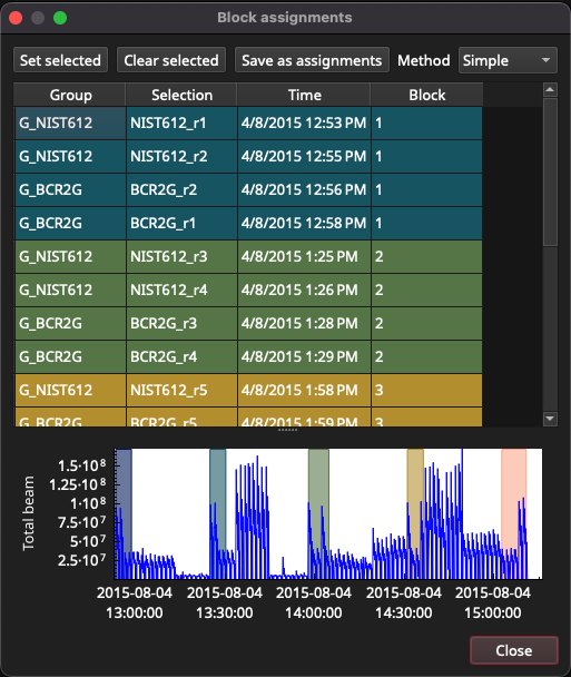
Fig. 32 A screenshot of the Block Setup window
After closing the 3DTE Setup window, it may take several seconds or up to a minute to finish the calculations.
In this experiment, Int Stds could be set in the same way as described in Setting Internal Standard values. Similarly, QAQC results for BHVO2G can be checked as described in Simple QAQC. At this point, the process for visualizing and exporting results are the same as the previous tutorials.
Conclusion
This concludes this guide to 3DTE data processing with Essentials. If you have any questions about this example, or about Essentials in general, please let us know at iolite’s support email, or on iolite’s forum.